Time Series Analysis with LSTM using Python’s Keras Library

Introduction
Time series analysis refers to the analysis of change in the trend of the data over a period of time. Time series analysis has a variety of applications. One such application is the prediction of the future value of an item based on its past values. Future stock price prediction is probably the best example of such an application. In this article, we will see how we can perform time series analysis with the help of a recurrent neural network. We will be predicting the future stock prices of the Apple Company (AAPL), based on its stock prices of the past 5 years.
Dataset
The data that we are going to use for this article can be downloaded from Yahoo Finance. For training our algorithm, we will be using the Apple stock prices from 1st January 2013 to 31 December 2017. For the sake of prediction, we will use the Apple stock prices for the month of January 2018. So in order to evaluate the performance of the algorithm, download the actual stock prices for the month of January 2018 as well.
Let’s now see how our data looks. Open the Apple stock price training file that contains data for five years. You will see that it contains seven columns: Date, Open, High, Low, Close, Adj Close and Volume. We will be predicting the opening stock price, therefore we are not interested in the rest of the columns.
If you plot the opening stock prices against the date, you will see the following plot:
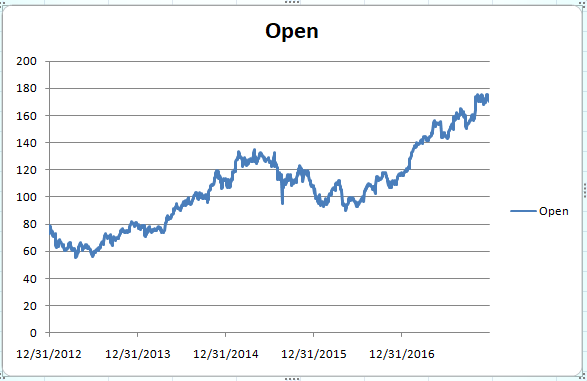
You can see that the trend is highly non-linear and it is very difficult to capture the trend using this information. This is where the power of LSTM can be utilized. LSTM (Long Short-Term Memory network) is a type of recurrent neural network capable of remembering the past information and while predicting the future values, it takes this past information into account.
Enough of the preliminaries, let’s see how LSTM can be used for time series analysis.
Predicting Future Stock Prices
Stock price prediction is similar to any other machine learning problem where we are given a set of features and we have to predict a corresponding value. We will perform the same steps as we do perform in order to solve any machine learning problem. Follow these steps:
Import Libraries
The first step, as always is to import the required libraries. Execute the following script to do so:
import numpy as np
import matplotlib.pyplot as plt
import pandas as pd
Import Dataset
Execute the following script to import the data set. For the sake of this article, the data has been stored in the Datasets folder, inside the “E” drive. You can change the path accordingly.
apple_training_complete = pd.read_csv(r'E:Datasetsapple_training.csv')
As we said earlier, we are only interested in the opening price of the stock. Therefore, we will filter all the data from our training set and will retain only the values for the Open column. Execute the following script:
apple_training_processed = apple_training_complete.iloc[:, 1:2].values
Data Normalization
As a rule of thumb, whenever you use a neural network, you should normalize or scale your data. We will use MinMaxScaler class from the sklear.preprocessing library to scale our data between 0 and 1. The feature_range parameter is used to specify the range of the scaled data. Execute the following script:
from sklearn.preprocessing import MinMaxScaler
scaler = MinMaxScaler(feature_range = (0, 1))

apple_training_scaled = scaler.fit_transform(apple_training_processed)
Convert Training Data to Right Shape
As I said earlier, in a time series problems, we have to predict a value at time T, based on the data from days T-N where N can be any number of steps. In this article, we are going to predict the opening stock price of the data based on the opening stock prices for the past 60 days. I have tried and tested different numbers and found that the best results are obtained when past 60 time steps are used. You can try different numbers and see how your algorithm performs.
Our feature set should contain the opening stock price values for the past 60 days while the label or dependent variable should be the stock price at the 61st day. Execute the following script to create feature and label set.
features_set = []
labels = []
for i in range(60, 1260):
    features_set.append(apple_training_scaled[i-60:i, 0])
    labels.append(apple_training_scaled[i, 0])
In the script above we create two lists: feature_set and labels. There are 1260 records in the training data. We execute a loop that starts from 61st record and stores all the previous 60 records to the feature_set list. The 61st record is stored in the labels list.
We need to convert both the feature_set and the labels list to the numpy array before we can use it for training. Execute the following script:
features_set, labels = np.array(features_set), np.array(labels)
In order to train LSTM on our data, we need to convert our data into the shape accepted by the LSTM. We need to convert our data into three-dimensional format. The first dimension is the number of records or rows in the dataset which is 1260 in our case. The second dimension is the number of time steps which is 60 while the last dimension is the number of indicators. Since we are only using one feature, i.e Open, the number of indicators will be one. Execute the following script:
features_set = np.reshape(features_set, (features_set.shape[0], features_set.shape[1], 1))
Training The LSTM
We have preprocessed our data and have converted it into the desired format. now is the time to create our LSTM. The LSTM model that we are going to create will be a sequential model with multiple layers. We will add four LSTM layers to our model followed by a dense layer that predicts the future stock price.
Let’s first import the libraries that we are going to need in order to create our model:
from keras.models import Sequential
from keras.layers import Dense
from keras.layers import LSTM
from keras.layers import Dropout
In the script above we imported the Sequential class from keras.models library and Dense, LSTM, and Dropout classes from keras.layers library.
As a first step, we need to instantiate the Sequential class. This will be our model class and we will add LSTM, Dropout and Dense layers to this model. Execute the following script
model = Sequential()
Creating LSTM and Dropout Layers
Let’s add LSTM layer to the model that we just created. Execute the following script to do so:
model.add(LSTM(units=50, return_sequences=True, input_shape=(features_set.shape[1], 1)))
To add a layer to the sequential model, the add method is used. Inside the add method, we passed our LSTM layer. The first parameter to the LSTM layer is the number of neurons or nodes that we want in the layer. The second parameter is return_sequences, which is set to true since we will add more layers to the model. The first parameter to the input_shape is the number of time steps while the last parameter is the number of indicators.
Let’s now add a dropout layer to our model. Dropout layer is added to avoid over-fitting, which is a phenomenon where a machine learning model performs better on the training data compared to the test data. Execute the following script to add dropout layer.
model.add(Dropout(0.2))
Let’s add three more LSTM and dropout layers to our model. Run the following script.
model.add(LSTM(units=50, return_sequences=True))
model.add(Dropout(0.2))

model.add(LSTM(units=50, return_sequences=True))
model.add(Dropout(0.2))

model.add(LSTM(units=50))
model.add(Dropout(0.2))
Creating Dense Layer
To make our model more robust, we add a dense layer at the end of the model. The number of neurons in the dense layer will be set to 1 since we want to predict a single value in the output.
model.add(Dense(units = 1))
Model Compilation
Finally, we need to compile our LSTM before we can train it on the training data. The following script compiles the our model.
model.compile(optimizer = 'adam', loss = 'mean_squared_error')
We call the compile method on the Sequential model object which is “model” in our case. We use the mean squared error as loss function and to reduce the loss or to optimize the algorithm, we use the adam optimizer.
Algorithm Training
Now is the time to train the model that we defined in the previous few steps. To do so, we call the fit method on the model and pass it our training features and labels as shown below:
model.fit(features_set, labels, epochs = 100, batch_size = 32)
Depending upon your hardware, model training can take some time.
Testing our LSTM
We have successfully trained our LSTM, now is the time to test the performance of our algorithm on the test set by predicting the opening stock prices for the month of January 2018. However, as we did with the training data, we need to convert our test data in the right format.
Let’s first import our test data. Execute the following script:
apple_testing_complete = pd.read_csv(r'E:Datasetsapple_testing.csv')
apple_testing_processed = apple_testing_complete.iloc[:, 1:2].values
In the above script, we import our test data and as we did with the training data, we removed all the columns from the test data except the column that contains opening stock prices.
If the opening stock prices for the month of January 2018 are plotted against the dates, you should see the following graph.
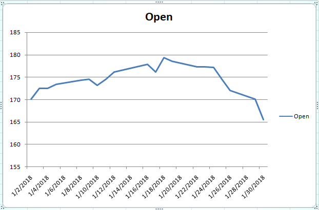
You can see that the trend is highly non-linear. Overall, the stock prices see small rise at the start of the month followed by a downward trend at the end of the month, with a slight increase and decrease in the stock prices in-between. It is extremely difficult to forecast such a trend. Let’s see if the LSTM we trained is actually able to predict such a trend.
Converting Test Data to Right Format
For each day of January 2018, we want our feature set to contain the opening stock prices for the previous 60 days. For the 1st of January, we need the stock prices for the previous 60 days. To do so, we need to concatenate our training data and test data before preprocessing. Execute the following script to do so:
apple_total = pd.concat((apple_training_complete['Open'], apple_testing_complete['Open']), axis=0)
Now let’s prepare our test inputs. The input for each day should contain the opening stock prices for the previous 60 days. That means we need opening stock prices for the 20 test days for the month of January 2018 and the 60 stock prices from the last 60 days for the training set. Execute the following script to fetch those 80 values.
test_inputs = apple_total[len(apple_total) - len(apple_testing_complete) - 60:].values
As we did for the training set, we need to scale our test data. Execute the following script:
test_inputs = test_inputs.reshape(-1,1)
test_inputs = scaler.transform(test_inputs)
We scaled our data, now let’s prepare our final test input set that will contain previous 60 stock prices for the month of January. Execute the following script:
test_features = []
for i in range(60, 80):
    test_features.append(test_inputs[i-60:i, 0])
Finally, we need to convert our data into the three-dimensional format which can be used as input to the LSTM. Execute the following script:
test_features = np.array(test_features)
test_features = np.reshape(test_features, (test_features.shape[0], test_features.shape[1], 1))
Making Predictions
Now is the time to see the magic. We preprocessed our test data and now we can use it to make predictions. To do so, we simply need to call the predict method on the model that we trained. Execute the following script:
predictions = model.predict(test_features)
Since we scaled our data, the predictions made by the LSTM are also scaled. We need to reverse the scaled prediction back to their actual values. To do so, we can use the ìnverse_transform method of the scaler object we created during training. Take a look at the following script:
predictions = scaler.inverse_transform(predictions)
Finally, let’s see how well did our algorithm predicted the future stock prices. Execute the following script:
plt.figure(figsize=(10,6))
plt.plot(apple_testing_processed, color='blue', label='Actual Apple Stock Price')
plt.plot(predictions , color='red', label='Predicted Apple Stock Price')
plt.title('Apple Stock Price Prediction')
plt.xlabel('Date')
plt.ylabel('Apple Stock Price')
plt.legend()
plt.show()
The output looks like this:
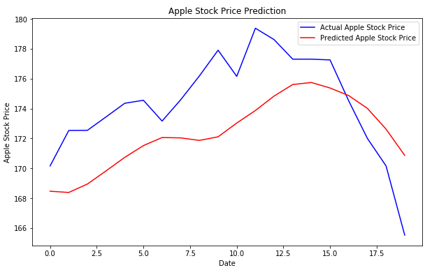
In the output, the blue line represents the actual stock prices for the month of January 2018, while the red line represents the predicted stock prices. You can clearly see that our algorithm has been able to capture the overall trend. The predicted prices also see a bullish trend at the beginning followed by a bearish or downwards trend at the end. Amazing, isn’t it?
Conclusion
A long short-term memory network (LSTM) is one of the most commonly used neural networks for time series analysis. The ability of LSTM to remember previous information makes it ideal for such tasks. In this article, we saw how we can use LSTM for the Apple stock price prediction. I would suggest that you download stocks of some other organization like Google or Microsoft from Yahoo Finance and see if your algorithm is able to capture the trends.