Implementing SVM and Kernel SVM with Python’s Scikit-Learn
A support vector machine (SVM) is a type of supervised machine learning classification algorithm. SVMs were introduced initially in 1960s and were later refined in 1990s. However, it is only now that they are becoming extremely popular, owing to their ability to achieve brilliant results. SVMs are implemented in a unique way when compared to other machine learning algorithms.
In this article we’ll see what support vector machines algorithms are, the brief theory behind support vector machine and their implementation in Python’s Scikit-Learn library. We will then move towards an advanced SVM concept, known as Kernel SVM, and will also implement it with the help of Scikit-Learn.
Simple SVM
In case of linearly separable data in two dimensions, as shown in Fig. 1, a typical machine learning algorithm tries to find a boundary that divides the data in such a way that the misclassification error can be minimized. If you closely look at Fig. 1, there can be several boundaries that correctly divide the data points. The two dashed lines as well as one solid line classify the data correctly.
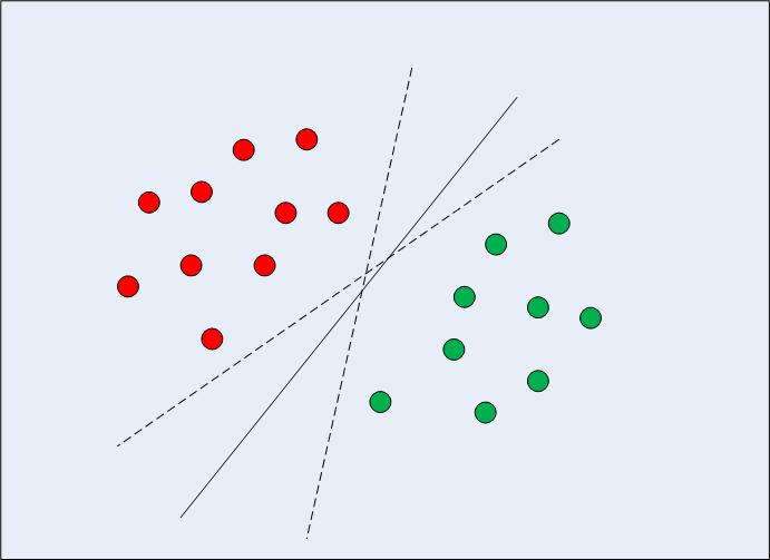
Fig 1: Multiple Decision Boundaries
SVM differs from the other classification algorithms in the way that it chooses the decision boundary that maximizes the distance from the nearest data points of all the classes. An SVM doesn’t merely find a decision boundary; it finds the most optimal decision boundary.
The most optimal decision boundary is the one which has maximum margin from the nearest points of all the classes. The nearest points from the decision boundary that maximize the distance between the decision boundary and the points are called support vectors as seen in Fig 2. The decision boundary in case of support vector machines is called the maximum margin classifier, or the maximum margin hyper plane.
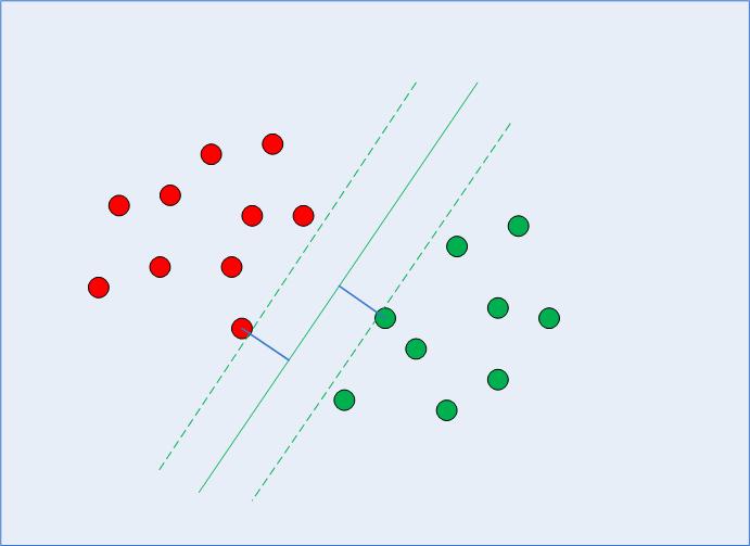
Fig 2: Decision Boundary with Support Vectors
There is complex mathematics involved behind finding the support vectors, calculating the margin between decision boundary and the support vectors and maximizing this margin. In this tutorial we will not go into the detail of the mathematics, we will rather see how SVM and Kernel SVM are implemented via the Python Scikit-Learn library.
Implementing SVM with Scikit-Learn
The dataset that we are going to use in this section is the same that we used in the classification section of the decision tree tutorial.
Our task is to predict whether a bank currency note is authentic or not based upon four attributes of the note i.e. skewness of the wavelet transformed image, variance of the image, entropy of the image, and curtosis of the image. This is a binary classification problem and we will use SVM algorithm to solve this problem. The rest of the section consists of standard machine learning steps.
Importing libraries
The following script imports required libraries:
import pandas as pd
import numpy as np
import matplotlib.pyplot as plt
%matplotlib inline
Importing the Dataset
The data is available for download at the following link:
https://drive.google.com/file/d/13nw-uRXPY8XIZQxKRNZ3yYlho-CYm_Qt/view
The detailed information about the data is available at the following link:
https://archive.ics.uci.edu/ml/datasets/banknote+authentication
Download the dataset from the Google drive link and store it locally on your machine. For this example the CSV file for the dataset is stored in the “Datasets” folder of the D drive on my Windows computer. The script reads the file from this path. You can change the file path for your computer accordingly.
To read data from CSV file, the simplest way is to use read_csv method of the pandas library. The following code reads bank currency note data into pandas dataframe:
bankdata = pd.read_csv("D:/Datasets/bill_authentication.csv")
Exploratory Data Analysis
There are virtually limitless ways to analyze datasets with a variety of Python libraries. For the sake of simplicity we will only check the dimensions of the data and see first few records. To see the rows and columns and of the data, execute the following command:
bankdata.shape
In the output you will see (1372,5). This means that the bank note dataset has 1372 rows and 5 columns.
To get a feel of how our dataset actually looks, execute the following command:
bankdata.head()
The output will look like this:
| Variance | Skewness | Curtosis | Entropy | Class | |
|---|---|---|---|---|---|
| 0 | 3.62160 | 8.6661 | -2.8073 | -0.44699 | 0 |
| 1 | 4.54590 | 8.1674 | -2.4586 | -1.46210 | 0 |
| 2 | 3.86600 | -2.6383 | 1.9242 | 0.10645 | 0 |
| 3 | 3.45660 | 9.5228 | -4.0112 | -3.59440 | 0 |
| 4 | 0.32924 | -4.4552 | 4.5718 | -0.98880 | 0 |
You can see that all of the attributes in the dataset are numeric. The label is also numeric i.e. 0 and 1.
Data Preprocessing
Data preprocessing involves (1) Dividing the data into attributes and labels and (2) dividing the data into training and testing sets.
To divide the data into attributes and labels, execute the following code:
X = bankdata.drop('Class', axis=1)
y = bankdata['Class']
In the first line of the script above, all the columns of the bankdata dataframe are being stored in the X variable except the “Class” column, which is the label column. The drop() method drops this column.
In the second line, only the class column is being stored in the y variable. At this point of time X variable contains attributes while y variable contains corresponding labels.
Once the data is divided into attributes and labels, the final preprocessing step is to divide data into training and test sets. Luckily, the model_selection library of the Scikit-Learn library contains the train_test_split method that allows us to seamlessly divide data into training and test sets.
Execute the following script to do so:
from sklearn.model_selection import train_test_split
X_train, X_test, y_train, y_test = train_test_split(X, y, test_size = 0.20)
Training the Algorithm
We have divided the data into training and testing sets. Now is the time to train our SVM on the training data. Scikit-Learn contains the svm library, which contains built-in classes for different SVM algorithms. Since we are going to perform a classification task, we will use the support vector classifier class, which is written as SVC in the Scikit-Learn’s svm library. This class takes one parameter, which is the kernel type. This is very important. In the case of a simple SVM we simply set this parameter as “linear” since simple SVMs can only classify linearly separable data. We will see non-linear kernels in the next section.
The fit method of SVC class is called to train the algorithm on the training data, which is passed as a parameter to the fit method. Execute the following code to train the algorithm:
from sklearn.svm import SVC
svclassifier = SVC(kernel='linear')
svclassifier.fit(X_train, y_train)
Making Predictions
To make predictions, the predict method of the SVC class is used. Take a look at the following code:
y_pred = svclassifier.predict(X_test)
Evaluating the Algorithm
Confusion matrix, precision, recall, and F1 measures are the most commonly used metrics for classification tasks. Scikit-Learn’s metrics library contains the classification_report and confusion_matrix methods, which can be readily used to find out the values for these important metrics.
Here is the code for finding these metrics:
from sklearn.metrics import classification_report, confusion_matrix
print(confusion_matrix(y_test,y_pred))
print(classification_report(y_test,y_pred))
Results
The evaluation results are as follows:
[[152    0]
 [  1  122]]
              precision   recall   f1-score   support

           0       0.99     1.00       1.00       152
           1       1.00     0.99       1.00       123

avg / total        1.00     1.00       1.00       275
From the results it can be observed that SVM slightly outperformed the decision tree algorithm. There is only one misclassification in the case of SVM algorithm compared to four misclassifications in the case of the decision tree algorithm.
Kernel SVM
In the previous section we saw how the simple SVM algorithm can be used to find decision boundary for linearly separable data. However, in the case of non-linearly separable data, such as the one shown in Fig. 3, a straight line cannot be used as a decision boundary.
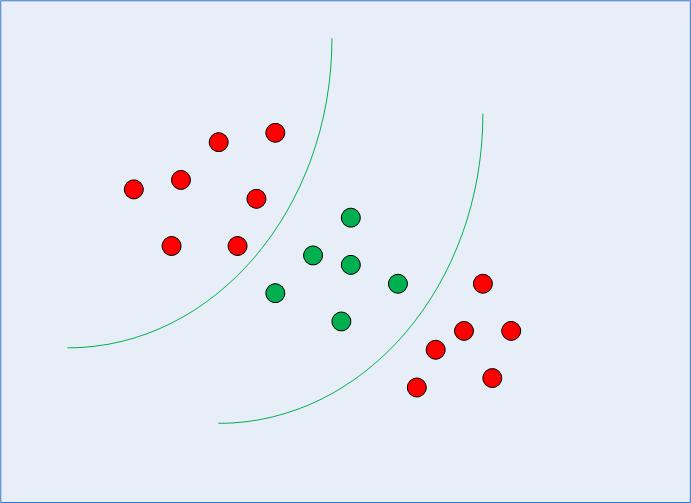
Fig 3: Non-linearly Separable Data
In case of non-linearly separable data, the simple SVM algorithm cannot be used. Rather, a modified version of SVM, called Kernel SVM, is used.
Basically, the kernel SVM projects the non-linearly separable data lower dimensions to linearly separable data in higher dimensions in such a way that data points belonging to different classes are allocated to different dimensions. Again, there is complex mathematics involved in this, but you do not have to worry about it in order to use SVM. Rather we can simply use Python’s Scikit-Learn library that to implement and use the kernel SVM.
Implementing Kernel SVM with Scikit-Learn
Implementing Kernel SVM with Scikit-Learn is similar to the simple SVM. In this section, we will use the famous iris dataset to predict the category to which a plant belongs based on four attributes: sepal-width, sepal-length, petal-width and petal-length.
The dataset can be downloaded from the following link:
https://archive.ics.uci.edu/ml/datasets/iris4
The rest of the steps are typical machine learning steps and need very little explanation until we reach the part where we train our Kernel SVM.
Importing Libraries
import numpy as np
import matplotlib.pyplot as plt
import pandas as pd
Importing the Dataset
url = "https://archive.ics.uci.edu/ml/machine-learning-databases/iris/iris.data"

# Assign colum names to the dataset
colnames = ['sepal-length', 'sepal-width', 'petal-length', 'petal-width', 'Class']

# Read dataset to pandas dataframe
irisdata = pd.read_csv(url, names=colnames)
Preprocessing
X = irisdata.drop('Class', axis=1)
y = irisdata['Class']
Train Test Split
from sklearn.model_selection import train_test_split
X_train, X_test, y_train, y_test = train_test_split(X, y, test_size = 0.20)
Training the Algorithm
To train the kernel SVM, we use the same SVC class of the Scikit-Learn’s svm library. The difference lies in the value for the kernel parameter of the SVC class. In the case of the simple SVM we used “linear” as the value for the kernel parameter. However, for kernel SVM you can use Gaussian, polynomial, sigmoid, or computable kernel. We will implement polynomial, Gaussian, and sigmoid kernels to see which one works better for our problem.
1. Polynomial Kernel
In the case of polynomial kernel, you also have to pass a value for the degree parameter of the SVC class. This basically is the degree of the polynomial. Take a look at how we can use a polynomial kernel to implement kernel SVM:
from sklearn.svm import SVC
svclassifier = SVC(kernel='poly', degree=8)
svclassifier.fit(X_train, y_train)
Making Predictions
Now once we have trained the algorithm, the next step is to make predictions on the test data.
Execute the following script to do so:
y_pred = svclassifier.predict(X_test)
Evaluating the Algorithm
As usual, the final step of any machine learning algorithm is to make evaluations for polynomial kernel. Execute the following script:
from sklearn.metrics import classification_report, confusion_matrix
print(confusion_matrix(y_test, y_pred))
print(classification_report(y_test, y_pred))
The output for the kernel SVM using polynomial kernel looks like this:
[[11  0  0]
 [ 0 12  1]
 [ 0  0  6]]
                 precision   recall   f1-score   support

    Iris-setosa       1.00     1.00       1.00        11
Iris-versicolor       1.00     0.92       0.96        13
 Iris-virginica       0.86     1.00       0.92         6

    avg / total       0.97     0.97       0.97        30
Now let’s repeat the same steps for Gaussian and sigmoid kernels.
2. Gaussian Kernel
Take a look at how we can use polynomial kernel to implement kernel SVM:
from sklearn.svm import SVC
svclassifier = SVC(kernel='rbf')
svclassifier.fit(X_train, y_train)
To use Gaussian kernel, you have to specify ‘rbf’ as value for the Kernel parameter of the SVC class.
Prediction and Evaluation
y_pred = svclassifier.predict(X_test)
from sklearn.metrics import classification_report, confusion_matrix
print(confusion_matrix(y_test, y_pred))
print(classification_report(y_test, y_pred))
The output of the Kernel SVM with Gaussian kernel looks like this:
[[11  0  0]
 [ 0 13  0]
 [ 0  0  6]]
                 precision   recall   f1-score   support

    Iris-setosa       1.00     1.00       1.00        11
Iris-versicolor       1.00     1.00       1.00        13
 Iris-virginica       1.00     1.00       1.00         6

    avg / total       1.00     1.00       1.00        30
3. Sigmoid Kernel
Finally, let’s use a sigmoid kernel for implementing Kernel SVM. Take a look at the following script:
from sklearn.svm import SVC
svclassifier = SVC(kernel='sigmoid')
svclassifier.fit(X_train, y_train)
To use the sigmoid kernel, you have to specify ‘sigmoid’ as value for the kernel parameter of the SVC class.
Prediction and Evaluation
y_pred = svclassifier.predict(X_test)
from sklearn.metrics import classification_report, confusion_matrix
print(confusion_matrix(y_test, y_pred))
print(classification_report(y_test, y_pred))
The output of the Kernel SVM with Sigmoid kernel looks like this:
[[ 0  0 11]
 [ 0  0 13]
 [ 0  0  6]]
                 precision   recall   f1-score   support

    Iris-setosa       0.00     0.00       0.00        11
Iris-versicolor       0.00     0.00       0.00        13
 Iris-virginica       0.20     1.00       0.33         6

    avg / total       0.04     0.20       0.07        30
Comparison of Kernel Performance
If we compare the performance of the different types of kernels we can clearly see that the sigmoid kernel performs the worst. This is due to the reason that sigmoid function returns two values, 0 and 1, therefore it is more suitable for binary classification problems. However, in our case we had three output classes.
Amongst the Gaussian kernel and polynomial kernel, we can see that Gaussian kernel achieved a perfect 100% prediction rate while polynomial kernel misclassified one instance. Therefore the Gaussian kernel performed slightly better. However, there is no hard and fast rule as to which kernel performs best in every scenario. It is all about testing all the kernels and selecting the one with the best results on your test dataset.
Resources
Want to learn more about SVMs, Scikit-Learn, and other useful machine learning algorithms? I’d recommend checking out some more detailed resources, like one of these books:
Conclusion
In this article we studied both simple and kernel SVMs. We studied the intuition behind the SVM algorithm and how it can be implemented with Python’s Scikit-Learn library. We also studied different types of kernels that can be used to implement kernel SVM. I would suggest you try to implement these algorithms on real-world datasets available at places like kaggle.com.
I would also suggest that you explore the actual mathematics behind the SVM. Although you are not necessarily going to need it in order to use the SVM algorithm, it is still very handy to know what is actually going on behind the scene while your algorithm is finding decision boundaries.